Table of Contents
Introduction to Rmarkdown
R Markdown allows you to create documents that serve as a neat record of your analysis. In the world of reproducible research, we want other researchers to easily understand what we did in our analysis, otherwise nobody can be certain that you analysed your data properly.
You might choose to create an RMarkdown document as an appendix to a paper or project assignment that you are doing, upload it to an online repository such as Github, or simply to keep as a personal record so you can quickly look back at your code and see what you did.
RMarkdown presents your code alongside its output (graphs, tables, etc.) with conventional text to explain it, a bit like a notebook. Just know that all the labs build were done in Rmarkdown!
For instance, have a look at this appendix for a Bachelor thesis which summarize neatly all the analysis that were carried out.
While it is not mandatory for your term paper we highly recommend that you use the Rmarkdown format for showing us your analysis!
Download Rmarkdown
You can download Rmarkdown as you would download any other R package:
install.packages('rmarkdown')
library(rmarkdown)
Create an Rmarkdown file
To create a new RMarkdown file (.Rmd), select File -> New File -> R Markdown..._ in RStudio, then choose the file type you want to create. For now we will focus on a .html Document, which can be easily converted to other file types later.
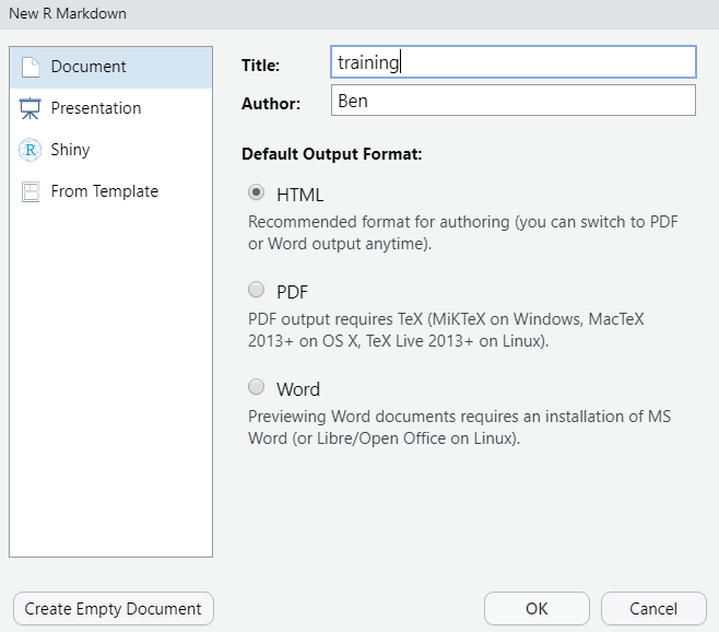
The newly created .Rmd file comes with basic instructions, but we want to create our own RMarkdown script, so go ahead and delete everything in the example file.
Now you can save the Rmd in a relevant folder.
YAML header
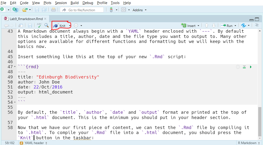
A Rmarkdown document always begin with a YAML header enclosed with ---. By default this includes a title, author, date and the file type you want to output to. Many other options are available for different functions and formatting but we will keep with the basics now.
Insert something like this at the top of your new .Rmd script:
By default, the title, author, date and output format are printed at the top of your .html document. This is the minimum you should put in your header section.
Now that we have our first piece of content, we can test the .Rmd file by compiling it to .html. To compile your .Rmd file into a .html document, you should press the Knit button in the taskbar:
By default, RStudio opens a separate preview window to display the output of your .Rmd file.
Code chunck
Below the YAML header is the space where you will write your code, accompanying explanation and any outputs. Code that is included in your .Rmd document should be enclosed by three backwards apostrophes ```. These are known as code chunks and look like this:
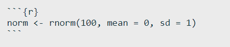
In your .html output, this should look like this:
norm <- rnorm(100, mean = 0, sd = 1)It’s important to remember when you are creating an RMarkdown file that if you want to run code that refers to an object, for example:
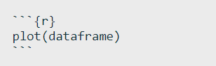
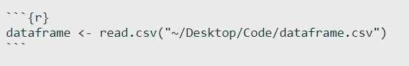
dataframe must refer to an object existing in your environment, thus if you want to load the dataset you want to analyze in the Rmd document you need to include the code in the .Rmd:
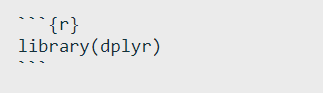
Similarly, if you are using any packages in your analysis, you will have to load them in the .Rmd file using library() as in a normal R script.
Hiding code chunk
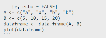
If you don’t want the code of a particular code chunk to appear in the final document, but still want to show the output (e.g. a plot), then you can include echo = FALSE in the code chunk instructions.
In some cases, when you load packages into RStudio, various warning messages such as “Warning: package ‘dplyr’ was built under R version 3.4.4” might appear. If you do not want these warning messages to appear, you can use warning = FALSE.

IMPORTANT: remember, R Markdown doesn’t pay attention to anything you have loaded in other R scripts, you MUST load all objects and packages in the R Markdown script.
Inserting figures
Inserting a graph into RMarkdown is easy, the more energy-demanding aspect might be adjusting the formatting.
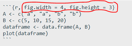
By default, RMarkdown will place graphs by maximising their height, while keeping them within the margins of the page and maintaining aspect ratio. If you have a particularly tall figure, this can mean a really huge graph. In the following example we modify the dimensions of the figure we created above. To manually set the figure dimensions, you can insert an instruction into the curly braces:
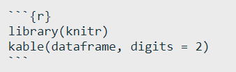
Inserting tables with kable()
The most aesthetically pleasing and simple table formatting function I have found is kable() in the knitr package. The first argument tells kable to make a table out of the object dataframe and that numbers should have two significant figures. Remember to load the knitr package in your .Rmd file as well.
Will return:
| A | B |
|---|---|
| a | 5 |
| a | 10 |
| b | 15 |
| b | 20 |
Formatting text
Markdown syntax can be used to change how text appears in your output file. Here are a few common formatting commands:
Italic
Bold
This is the code
Header 1
Header 2
- Unordered list item
- Unordered list item 2
- Unordered list item
- Unordered list item 2
Creating pdf documents in Rmarkdown
To compile a .pdf instead of a .html document, change output: from html_document to pdf_document in the YAML header:
Have a go yourself!
At this point you should be able to make your own document in Rmarkdown and show your entire analysis! Have a go and try to convert one of your r script into a Rmd document!