Table of Contents
This is now the last exercise on data vizualisation
Correction exercise
First, as in any other exercise I load the dataset in my environment. The dataset is a .rda file. .rda a basically a saved R object. Saving an R object is especially useful when you want to save the outpus of a statistical model which ran for days (or weeks).
We also load the package tidyverse as it contains most of the functions we will need for the analysis.
# Load the library
library(tidyverse)

# Load the dataset
load("C:/Users/benjamcr/Rproj/GEOG3006/data/ncbikecrash.rda")
data <- ncbikecrash # Store the ncbikecrash object in `data`
# See what you have in your dataset:
head(data)
# I do not show the output here as it is too long
There is a lot of data in this data and this might hinder our ability to read well this dataset … We will use the function filter() to get a clearer picture of the dataset.
Question 1: Run View(ncbikecrash) in your Console to view the data in the data viewer. What does each row in the dataset represent?
View(ncbikecrash)Each row of the dataset represent a single accident between a car driver and a bicyclist. In this dataset there is a lot of characteristics regarding the bicyclist (her / his age, sex, …), the same holds regarding the car driver.
min(data$crash_year)
[1] 2007
max(data$crash_year)
[1] 2014The timespan of the dataset is of 7 years, this is a consequent time series and a lot can be done with it.
Note that, like in the previous labs, this is a real dataset!
Question 2: How many bike crashes were recorded in NC between 2007 and 2014? How many variables are recorded on these crashes?
We have previsouly said that each row of the dataset represents an accident. There is therefore 7467 accidents. Nevertheless it is worth checking … In some cases your dataset will have mistakes and a row can be replicated. We can verify this by using the functions length and unique.
length(unique(data$object_id))
[1] 7467The result is 7467, there is no duplicates.
The function unique look at the unique different values contains in your vector. length returns the length of your vector.
Regarding the variables we can see that we have 66 variables recorded.
ncol(data)
[1] 66Question 3: How many bike crashes occurred in residential development areas where the driver was between 0 and 19 years old?
Here two columns are of interest for us:
development: variable which represents the “type” of area. Multiple categories are contain in this variables. In our case we are interested in the categoryresidential.
unique(data$development)
[1] "Farms, Woods, Pastures" "Residential"
[3] "Commercial"             "Institutional"
[5] "Industrial" driver_age_group: variable which represents the age category of the driver
We will first create a new dataset isolating these two variables, so we can have a clearer overview. We do that using the function select. The we will filter the observations corresponding to the criterions above. You are already familiar with the function which will do that for u: filter():
data_sub <- data %>%
  # First select the columns
  dplyr::select(development, driver_age_group)
head(data_sub) # This looks less messy!
# A tibble: 6 x 2
  development            driver_age_group
  <chr>                  <chr>
1 Farms, Woods, Pastures 30-39
2 Residential            <NA>
3 Farms, Woods, Pastures 30-39
4 Commercial             50-59
5 Residential            25-29
6 Farms, Woods, Pastures 0-19
# Now we filter the observations corresponding to our criterions
data_sub_filter <- data_sub %>%
  dplyr::filter(development == "Residential") %>%
  dplyr::filter(driver_age_group == "0-19")

# We can then compute the number of observations for the
# last dataset:
nrow(data_sub_filter)
[1] 223From the lines of codes above we can see that 223 accidents occurred in a residential area and were caused by a driver belonging to the age group 0-19.
(223 / 7467)*100
[1] 2.986474This represents more or less 3% of the total number of accidents
Question 4: Create a frequency table of the estimated speed of the car (driver_est_speed) involved in the crash. What is the most common estimated speed range in the dataset?
Here we will use the combination of the functions group_by and summarise. We first group_by the speed and summarise the number of accidents per speed class. Finally we make a nice lollipop chart.
data %>%
  dplyr::group_by(driver_est_speed) %>%
  dplyr::summarise(n = n()) %>%
  ggplot(., aes(x = driver_est_speed, y = n)) +
  geom_point(size = 3, color = "#a25079") +
  geom_segment(aes(x = driver_est_speed, xend = driver_est_speed, y=0, yend = n), color = "grey") +
  coord_flip() +
  theme_classic() +
  ylab("Number of accident") +
  xlab("Speed")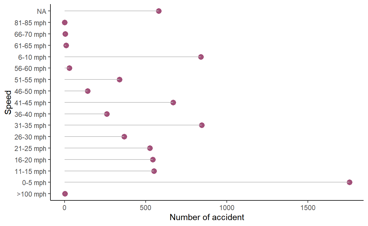
Finally, we can make this plot even better by ordering the plot (i.e. larger number of accidents to the smallest). For that we can use a function you didn’t see yet: reorder(). We will also get rid of the NA by using the function drop_na.
data %>%
  dplyr::group_by(driver_est_speed) %>%
  dplyr::summarise(n = n()) %>%
  drop_na() %>%
  ggplot(., aes(x = reorder(driver_est_speed, n), y = n)) +
  geom_point(size = 3, color = "#a25079") +
  geom_segment(aes(x = driver_est_speed, xend = driver_est_speed, y=0, yend = n), color = "grey") +
  coord_flip() +
  theme_classic() +
  ylab("Number of accident") +
  xlab("Speed")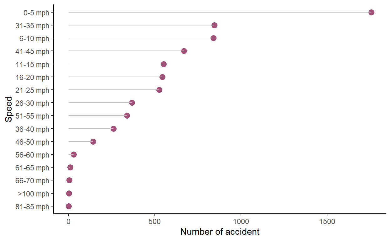
You can see that most accidents occur when the car is very slow - between 0 - 8km/h!
A last word on data wrangling and data visualization
Wrangling / Manipulating data and visualizing it requires a lot of training and these exercises alone won’t give you profitient skills. I have been using R for 3 years almost every day and I still make a lots of mistakes and I am constently ggogle-ing my problems.
My only advice is too stay consistent and to keep training. In this exercise and in during the previous ones I have introduced you to different dataset which are from real sources and which are very interesting. You should keep training with them, use the functions you have learned and try out different visualization methods (see the links below)
What is the next step: modelling! 🚀
In the next block of this course you will be introduced to the very important topics of modelling and statistical inference for making data-based conclusions. We will discuss building, interpreting, and selecting models, visualizing interaction effects, and prediction and model validation.
Statistical modelling has been a major tool for making rigorous conclusions about your data and making inferences about the world that surrounds you.
Additional ressources
Here are some books and website I recommend for improving you data visualisation skills. Data visualization is really fun and it is a great tool for communicating your results to a wide range of audiences!
- data-to-viz: This website is a gold mine for data visualization. It will help you decide which plot you should use for which type of data
- Fundamental of Data Visualization: A great book about the theory of data visualization. And it’s free!