Table of Contents
Exercise correction
First of all, we need to open the dataset.
nobel <- read.csv('C:/Users/benjamcr/Rproj/GEOG3006/data/nobel.csv')
head(nobel)
  id      firstname   surname year category
1  1 Wilhelm Conrad  Röntgen 1901  Physics
2  2     Hendrik A.   Lorentz 1902  Physics
3  3         Pieter    Zeeman 1902  Physics
4  4          Henri Becquerel 1903  Physics
5  5         Pierre     Curie 1903  Physics
6  6          Marie     Curie 1903  Physics
                                                                                                      affiliation
1                                                                                               Munich University
2                                                                                               Leiden University
3                                                                                            Amsterdam University
4                                                                                            École Polytechnique
5 École municipale de physique et de chimie industrielles (Municipal School of Industrial Physics and Chemistry)
6                                                                                                            <NA>
       city     country  born_date  died_date gender  born_city
1    Munich     Germany 1845-03-27 1923-02-10   male  Remscheid
2    Leiden Netherlands 1853-07-18 1928-02-04   male     Arnhem
3 Amsterdam Netherlands 1865-05-25 1943-10-09   male Zonnemaire
4     Paris      France 1852-12-15 1908-08-25   male      Paris
5     Paris      France 1859-05-15 1906-04-19   male      Paris
6      <NA>        <NA> 1867-11-07 1934-07-04 female     Warsaw
  born_country born_country_code  died_city died_country
1      Germany                DE     Munich      Germany
2  Netherlands                NL       <NA>  Netherlands
3  Netherlands                NL  Amsterdam  Netherlands
4       France                FR       <NA>       France
5       France                FR      Paris       France
6       Poland                PL Sallanches       France
  died_country_code overall_motivation share
1                DE               <NA>     1
2                NL               <NA>     2
3                NL               <NA>     2
4                FR               <NA>     2
5                FR               <NA>     4
6                FR               <NA>     4
                                                                                                                                                      motivation
1                            "in recognition of the extraordinary services he has rendered by the discovery of the remarkable rays subsequently named after him"
2                       "in recognition of the extraordinary service they rendered by their researches into the influence of magnetism upon radiation phenomena"
3                       "in recognition of the extraordinary service they rendered by their researches into the influence of magnetism upon radiation phenomena"
4                                                   "in recognition of the extraordinary services he has rendered by his discovery of spontaneous radioactivity"
5 "in recognition of the extraordinary services they have rendered by their joint researches on the radiation phenomena discovered by Professor Henri Becquerel"
6 "in recognition of the extraordinary services they have rendered by their joint researches on the radiation phenomena discovered by Professor Henri Becquerel"
        born_country_original     born_city_original
1       Prussia (now Germany) Lennep (now Remscheid)
2             the Netherlands                 Arnhem
3             the Netherlands             Zonnemaire
4                      France                  Paris
5                      France                  Paris
6 Russian Empire (now Poland)                 Warsaw
  died_country_original died_city_original city_original
1               Germany             Munich        Munich
2       the Netherlands               <NA>        Leiden
3       the Netherlands          Amsterdam     Amsterdam
4                France               <NA>         Paris
5                France              Paris         Paris
6                France         Sallanches          <NA>
  country_original
1          Germany
2  the Netherlands
3  the Netherlands
4           France
5           France
6             <NA>
Question 1: How many observations and how many variables are in the dataset?
We can use the functions nrow and ncol to get the number of observations and the number of variables in a dataset. As you may remember from the tutorials, the rows of a dataset are the observations (Tor, Gus or Lena in the kids_frame dataset for instance). The columns are the variables (names, shirt_color or height in the kids_frame dataset)
# Number of observations
nrow(nobel)
[1] 935
# Number of variables
ncol(nobel)
[1] 26Question 2: How many woman won a nobel price? How many men?
Although there is multiple ways of answering this question in R, a fast and efficient way of doing so is to use the combination group_by and summarise(), functions included in the dplyr package.
library(tidyverse)

nobel %>%
  dplyr::group_by(gender) %>%
  dplyr::summarise(n = n())
# A tibble: 3 x 2
  gender     n
  <chr>  <int>
1 female    52
2 male     856
3 org       27
In the line above I load the library
tidyverse. Later in the document we will see what is this library and why it is so useful.
From the output we can see that only 52 women got a nobel price while 856 men got a nobel price.
We can calculate the percentage of women who got a nobel price:
[1] 0.05726872Only 5%!
Question 3: Create a new data frame called nobel_living that filters for
- laureates for whom country is available (you can use the function
drop_na(), look on google what it does!) - females laureates who are still alive (their died_date is NA)
Here, we need to create a new object that we will call nobel_living. To select the data we are supposed to place in this dataset we will use the function filter, again from the dplyr package.
nobel_living <- nobel %>%
  drop_na(country) %>%
  filter(gender == "female") %>%
  filter(is.na(died_date))
The code above has three steps. Note that in this case there is no special order for the steps.
- First, I filter only for the laureates whom country is available with the function
drop_na - Then I filter only for laureates whom gender is
female - Finally, I filter only for the laureates whom died_date is
NA. Here I combine 2 functions:filterandis.na().
The function is.na() will test whether a particular cell value is NA or not. Here, if NA is true (the person is still living) then the function will filter for it. Roughly, you can translate this line of code by Filter the laureates whom died_date is NA.
Note that you can filter only the dead persons by adding a ! before the
is.na()function.
nobel_living <- nobel %>%
  drop_na(country) %>%
  filter(gender == "female") %>%
  filter(is.na(died_date))
We can translate this as Filter the laureates whom died_date is no NA.
Question 4: With this new dataset, summarize the number of females laureate who are still alive by country and make a histogram of the number of female laureates per country. Your histogram should include a title and title for the axis.
First, we will create a dataset which summarise the number of female laureates by country:
nobel_female_country <- nobel_living %>%
  group_by(country) %>%
  summarise(n = n())
This dataset should have 7 observations and only two variables which are n the number of living female laureate per country and country.
Then we can build our visualisation with the package ggplot2. Here I do not build a histogram but rather a lollipop chart.
nobel_female_country %>%
  ggplot(., aes(x = country, y = n)) +
  geom_point(size = 3, color = "#a25079") +
  geom_segment(aes(x = country, xend = country, y=0, yend = n), color = "grey") +
  coord_flip() +
  theme_minimal() +
  labs(title = "Number of nobel prices per country",
       xlab = "Number of nobel prices",
       ylab = "Country")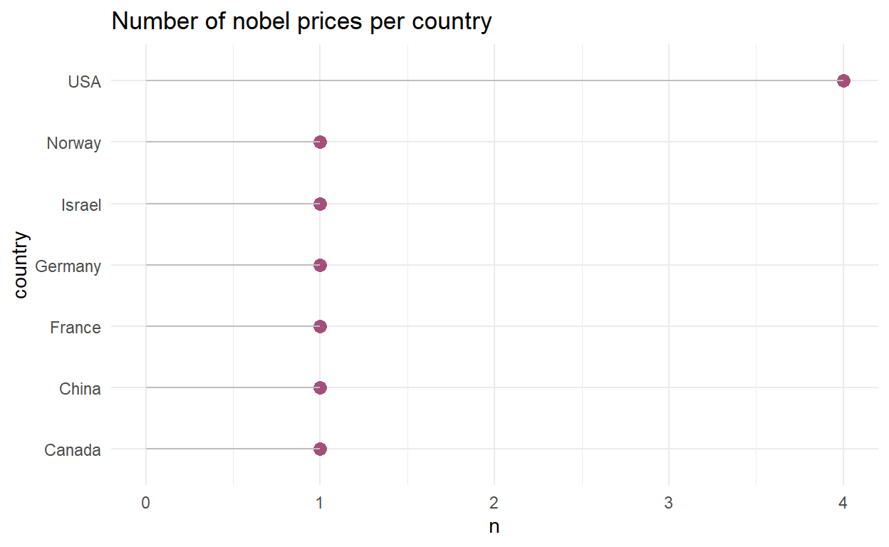
Question 5: Which country has the most female laureates?
From the lollipop chart we draw we can clearly see that the US has the most female living laureate. Note that Norway has a woman who won a Nobel Price and who is still alive, in fact May-Britt Moser works at NTNU in St-Olav!
A word on the tidyverse library
Previously, I have used the Tidyverse package which is a collection of R packages that share an underlying design philosophy, grammar and data structures.
We have already been using some of the packages included in the tidyverse including dplyr, magritrr (package which has the pipe) and ggplot2. There is a lot more to explore and a lot of very useful functions in it. Of course I do not know everything from the tidyverse and later in this course you may find more efficient ways to wrangle the data than I do, let me know if that’s the case!
I highly recommend to install the tidyverse package and to load it at the beginning of your script. If you do that you won’t have to load ggplot, dplyr … every time.
install.packages('tidyverse')
library(tidyverse)
If you want to improve your data science skills you can find some tips here.
Other functions that will make your life easier in R
You already have been introduced to some of the main functions from the dplyr package:
filtergroup_bysummarise
There is two other functions which will help you in your data analysis workflow, namely select() and mutate()
A few words on select()
It’s not uncommon to get datasets with hundreds or even thousands of variables. In this case, the first challenge is often narrowing in on the variables you’re actually interested in. select() allows you to rapidly zoom in on a useful subset using operations based on the names of the variables.
select() is not very useful on the kids_frame dataset but you can still get the idea:
# We reconstruct the kids_frame dataset
kids_frame <- data.frame(
  names = c("Tor", "Gus", "Bob", "Di", "Lena", "Tony", "Ingrid", "Maria", "Ed", "Raghnild"),
  height = c(110, 130, 115, 140, 125, 135, 120, 130, 130, 115),
  shirt_color = c("green", "green", "green", "blue", "blue", "green", "blue", "green", "green", "blue"),
  shoe_color = c("blue", "red", "grey", "blue", "pink", "red", "grey", "pink", "pink", "blue"),
  sex = c("m", "m", "m", "f", "f", "m", "f", "f", "m", "f"),
  age = c(8,11,8,12,11,11,9,12,12,8))
Imagine you would like to create a new dataset with only the columns names and height, with the select() function you would write:
kids_selected <- kids_frame %>%
  dplyr::select(names, height)

head(kids_selected)
  names height
1   Tor    110
2   Gus    130
3   Bob    115
4    Di    140
5  Lena    125
6  Tony    135
Now you reduced the initial dataset to only two columns.
A few words on mutate()
Besides selecting sets of existing columns, it’s often useful to add new columns that are functions of existing columns. That’s the job of mutate().
mutate() always adds new columns at the end of your dataset so we’ll start by creating a narrower dataset so we can see the new variables. Remember that when you’re in RStudio, the easiest way to see all the columns is View()
Here I will create a new column about the kids’ favorite food:
  names height shirt_color shoe_color sex age   fav_food
1   Tor    110       green       blue   m   8 strawberry
2   Gus    130       green        red   m  11      candy
3   Bob    115       green       grey   m   8      pasta
4    Di    140        blue       blue   f  12  chocolate
5  Lena    125        blue       pink   f  11      candy
6  Tony    135       green        red   m  11       beef
Now you can see that the new column has been created!
Other functions worth mentioning
Now you know the main functions of the tidyverse package that will allow you to wrangle efficiently. The list is not exhaustive and as I said I do not know all the functions! However here a small list of the tidyverse functions worth mentionning. You can look them up in R by typing ?NAME_FUNCTION or on google.
transmuterenamestarts_withends_withslice- …
For next lab
During next lab we will finish the bloc on Data visualisation and data wrangling. We will mainly repeat what we have been doing, using the same functions.
First, download the dataset here:
As you may see, this is an .rda file. A .rda file is basically a compressed R file. I saved this file in the folder “data”. TO open it I should write:
load("data/ncbikecrash.rda")You will use what you learned form the previous labs and answer these questions:
Question 1: Run View(ncbikecrash) in your Console to view the data in the data viewer. What does each row in the dataset represent?
Question 2: How many bike crashes were recorded in NC between 2007 and 2014? How many variables are recorded on these crashes?
Question 3: How many bike crashes occurred in residential development areas where the driver was between 0 and 19 years old?
Question 4: Create a frequency table of the estimated speed of the car (driver_est_speed) involved in the crash. What is the most common estimated speed range in the dataset?
Good luck!