Table of Contents
Introduction to data vizualisation
Being able to create visualizations (graphical representations) of data is a key step in being able to finding patterns in your data and communicate information and findings to others. In this lab you will learn to use the R library ggplot2. ggplot2 is a very powerful library which make us build beautiful plots with few lines of code. ggplot2 librar implements the Gramar of Graphics.
Learning this library will allow you to make nearly any kind of (static) data visualization, customized to your exact specifications. Learning this package will tremendously improve the way you understand your data.
Install and load the package
First of all you need to install the library ggplot2 with the following lines of code:
install.packages('ggplot2')And load the library:
library(ggplot2)Dataset
In this lab I will extend and use the dataset Thomas created during his lecture. You can copy the dataset to reproduce the graph of this lab.
kids_frame <- data.frame(
  names = c("Tor", "Gus", "Bob", "Di", "Lena", "Tony", "Ingrid", "Maria", "Ed", "Raghnild"),
  height = c(110, 130, 115, 140, 125, 135, 120, 130, 130, 115),
  shirt_color = c("green", "green", "green", "blue", "blue", "green", "blue", "green", "green", "blue"),
  shoe_color = c("blue", "red", "grey", "blue", "pink", "red", "grey", "pink", "pink", "blue"),
  sex = c("m", "m", "m", "f", "f", "m", "f", "f", "m", "f"),
  age = c(8,11,8,12,11,11,9,12,12,8))
You can check your dataset with the commands you learnt during the tutorial:
summary(kids_frame)
     names       height      shirt_color shoe_color sex
 Bob    :1   Min.   :110.0   blue :4     blue:3     f:5
 Di     :1   1st Qu.:116.2   green:6     grey:2     m:5
 Ed     :1   Median :127.5               pink:3
 Gus    :1   Mean   :125.0               red :2
 Ingrid :1   3rd Qu.:130.0
 Lena   :1   Max.   :140.0
 (Other):4
      age
 Min.   : 8.00
 1st Qu.: 8.25
 Median :11.00
 Mean   :10.20
 3rd Qu.:11.75
 Max.   :12.00
head(kids_frame)
  names height shirt_color shoe_color sex age
1   Tor    110       green       blue   m   8
2   Gus    130       green        red   m  11
3   Bob    115       green       grey   m   8
4    Di    140        blue       blue   f  12
5  Lena    125        blue       pink   f  11
6  Tony    135       green        red   m  11
The Grammar of Graphics
Just as the grammar of language helps us construct meaningful sentences out of words, the Grammar of Graphics helps us to construct graphical figures out of different visual elements. This grammar gives us a way to talk about parts of a plot: all the circles, lines, arrows, and words that are combined into a diagram for visualizing data. The Grammar of Graphics was adapted by Hadley Wickham to describe the components of a plot, including
- the data being plotted
- the geometrc objects (circles, lines, etc. ) that appear on the plot
- a set of mappings from variables in the data to the aesthetics (appearance) of the geometric objects
- a position adjustment for locating each geometric object on the plot
- a scale (e.g., range of values) for each aesthetic mapping used
- a coordinate system used to organize the geometric objects
- the facets or groups of data shown in different plots
Following this grammar, you can think of each plot as a set of layers of images, where each image’s appearance is based on some aspect of the data set. If this seems a bit theoric for now, it is normal. It looks much simpler when we code the plot.
The basics
In order to create a plot, you:
- Call the ggplot() function which creates a blank canvas
- Specify aesthetic mappings, which specifies how you want to map variables to visual aspects. In this case we are simply mapping the displ and hwy variables to the x- and y-axes.
- You then add new layers that are geometric objects which will show up on the plot. In this case we add geom_point to add a layer with points (dot) elements as the geometric shapes to represent the data.
For instance, here we will explore whether height depends on age:
# Initiate the plot
ggplot(data = kids_frame)

# Mapping the variable of interest
ggplot(data = kids_frame, aes(x = age, y = height))

# Finally, plot the data
ggplot(data = kids_frame, aes(x = age, y = height)) +
  geom_point()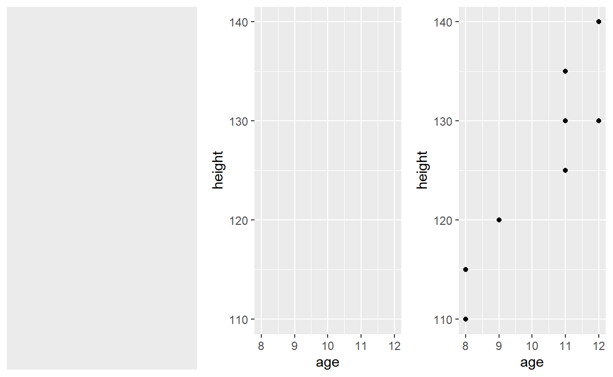
Note that when you added the geom layer you used the addition (+) operator. As you add new layers you will always use + to add onto your visualization.
Aesthetic Mappings
The aesthetic mappings take properties of the data and use them to influence visual characteristics, such as position, color, size, shape, or transparency. Each visual characteristic can thus encode an aspect of the data and be used to convey information.
All aesthetics for a plot are specified in the aes() function call (later in this tutorial you will see that each geom layer can have its own aes specification). For example, we can add a mapping the sex of the kid to a color characteristic:
ggplot(data = kids_frame, aes(x = age, y = height, color = sex)) +
  geom_point()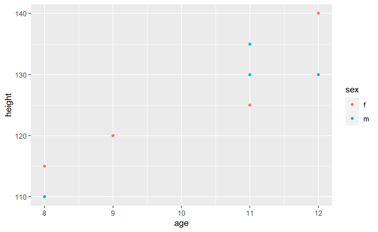
Note that using the aes() function will cause the visual channel to be based on the data specified in the argument. For instance, if you want all your points to be green you need to specify it outside the aesthetics:
ggplot(data = kids_frame, aes(x = age, y = height)) +
  geom_point(color = "green")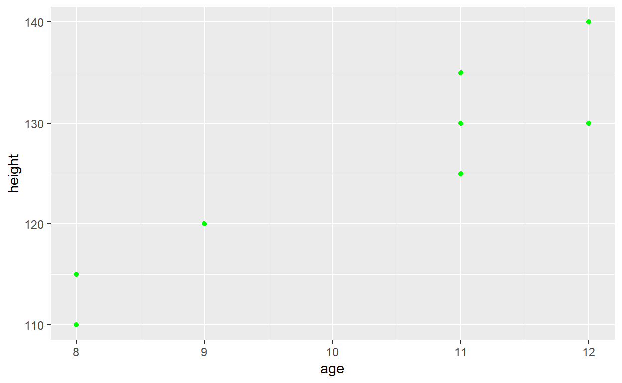
Specifying Geometric Shapes
Building on these basics, ggplot2 can be used to build almost any kind of plot you may want. These plots are declared using functions that follow from the Grammar of Graphics.
The most obvious distinction between plots is what geometric objects (geoms) they include. ggplot2 supports a number of different types of geoms. The most important geoms are:
geom_pointfor drawing individual points (e.g., a scatter plot)geom_linefor drawing lines (e.g., for a line charts)geom_smoothfor drawing smoothed lines (e.g., for simple trends or approximations)geom_barfor drawing bars (e.g., for bar charts)geom_histogramfor drawing binned values (e.g. a histogram)geom_boxplotfor drawing a boxplot
Note that geom_bar and geom_histogram do not require the mapping of a y:
ggplot(data = kids_frame, aes(x = age, y = height)) +
  geom_point()

ggplot(data = kids_frame, aes(x = age, y = height)) +
  geom_line()

ggplot(data = kids_frame, aes(x = height)) +
  geom_histogram()

ggplot(data = kids_frame, aes(x = sex, y = height)) +
  geom_boxplot()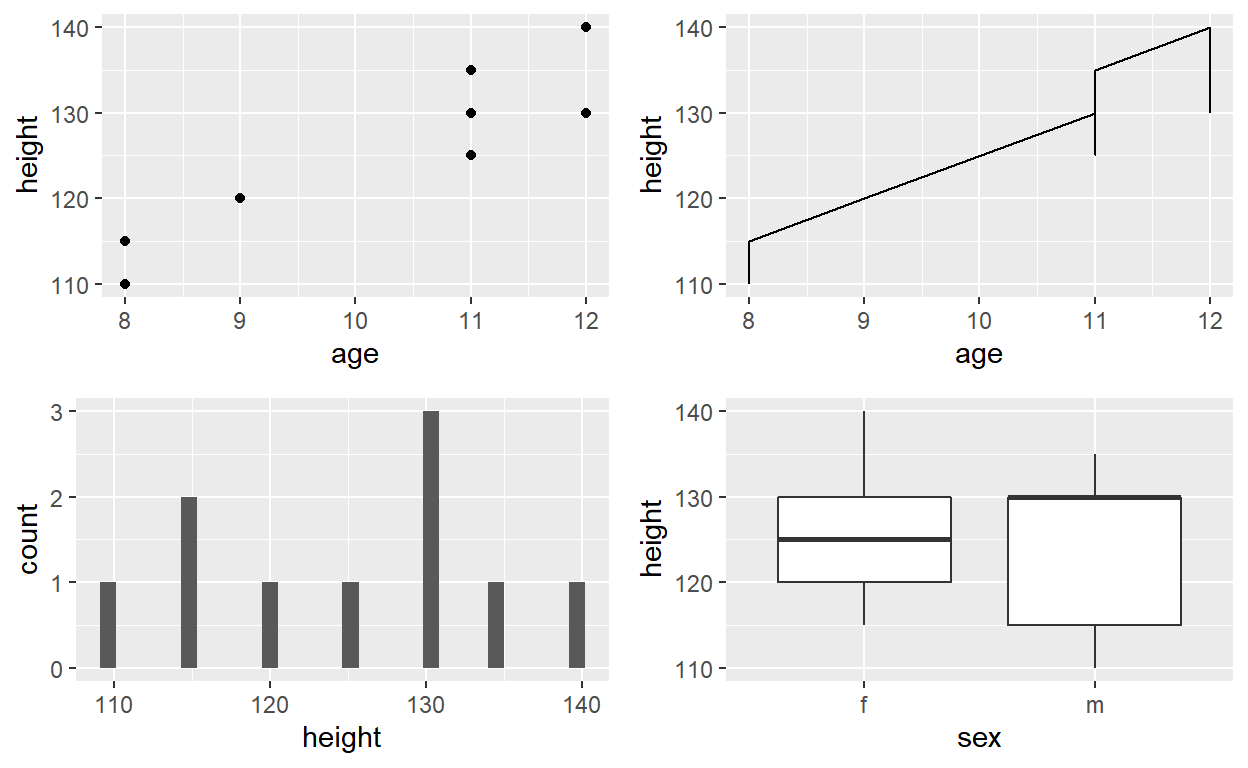
But what makes ggplot and the Grammar of Graphics really powerful is that you can add multiple geometries to a plot, thus allowing you to create complex graphics showing multiple aspects of your data.
For instance, if I want to vizualise more clearly the trend between age and height I can add a geom_smooth:
ggplot(data = kids_frame, aes(x = age, y = height)) +
  geom_point() +
  geom_smooth()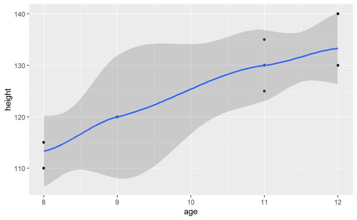
Position adjustments
In addition to a default statistical transformation, each geom also has a default position adjustment which specifies a set of “rules” as to how different components should be positioned relative to each other. This position is noticeable in a geom_bar if you map a different variable to the color visual characteristic:
ggplot(data = kids_frame, aes(x = sex, fill = shoe_color)) +
  geom_bar()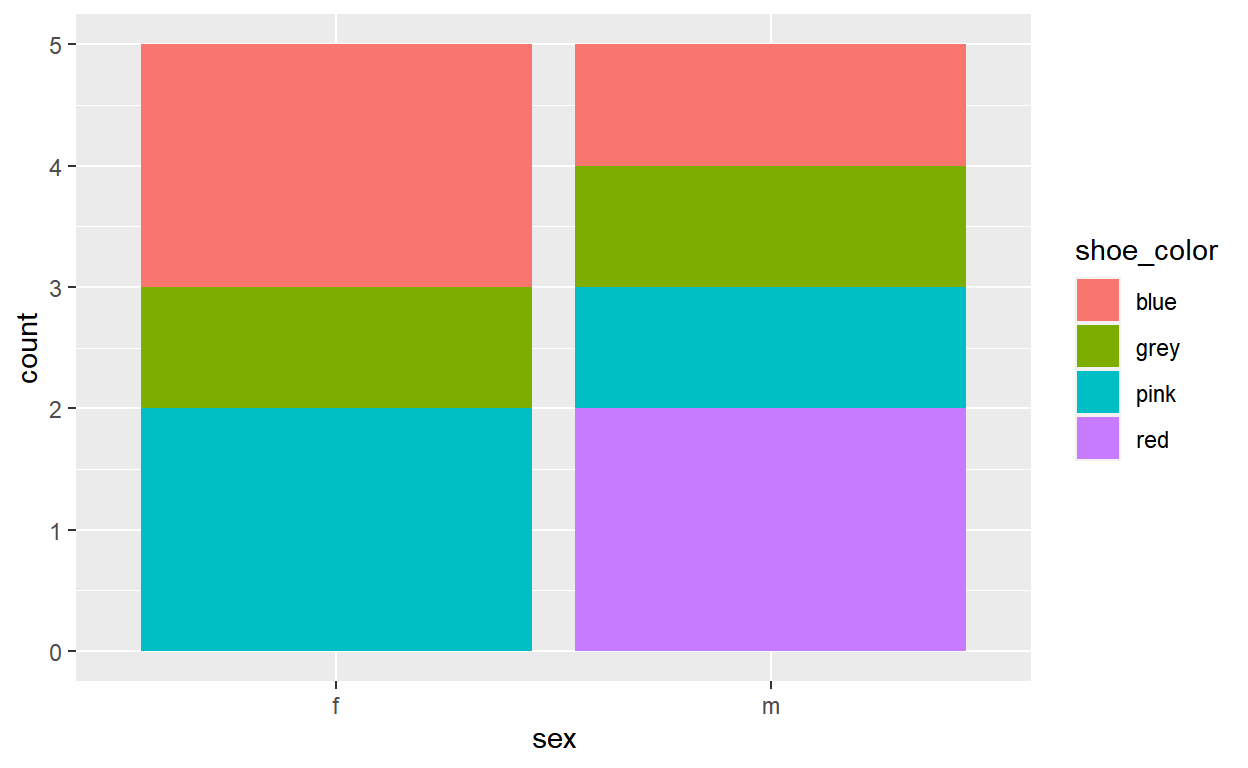
The geom_bar by default uses a position adjustment of “stack”, which makes each rectangle’s height proportional to its value and stacks them on top of each other. We can use the position argument to specify what position adjustment rules to follow:
ggplot(data = kids_frame, aes(x = sex, fill = shoe_color)) +
  geom_bar(position = "dodge")

ggplot(data = kids_frame, aes(x = sex, fill = shoe_color)) +
  geom_bar(position = "fill")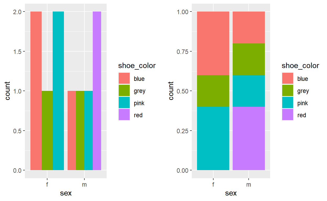
Check the documentation for each particular geom to learn more about its positioning adjustments.
Managing scale
Whenever you specify an aesthetic mapping, ggplot uses a particular scale to determine the range of values that the data should map to.
While the default scales will work fine, it is possible to explicitly add different scales to replace the defaults. This is especially useful for the colors. While you can use the default coloring, a more common option is to leverage the pre-defined palettes from colorbrewer.org. Here is an overview of the palette and their names.
These color sets have been carefully designed to look good and to be viewable to people with certain forms of color blindness. We can change the colors by specifying a palette argument in the scale_color_brewer().
ggplot(data = kids_frame, aes(x = age, y = height, color = names)) +
  geom_point(size = 3)

ggplot(data = kids_frame, aes(x = age, y = height, color = names)) +
  geom_point(size = 3) +
  scale_color_brewer(palette = "Set3")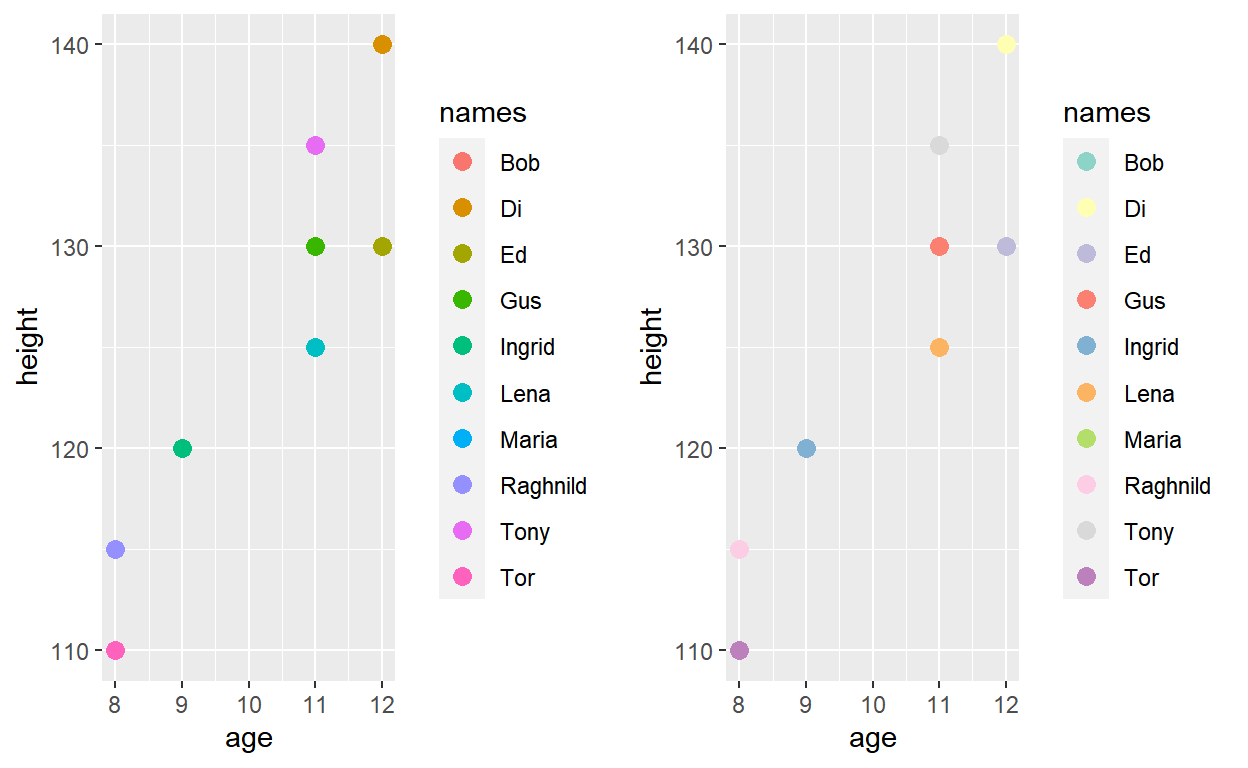
Facets
Facets are ways of grouping a data plot into multiple different pieces (subplots). This allows you to view a separate plot for each value in a categorical variable. This is very useful when you want to evaluate the patterns in different categories in your data. You can construct a plot with multiple facets by using the facet_wrap() function. This will produce a “row” of subplots, one for each categorical variable (the number of rows can be specified with an additional argument):
ggplot(data = kids_frame, aes(x = age, y = height, color = names)) +
  geom_point(size = 3) +
  facet_wrap( ~ sex)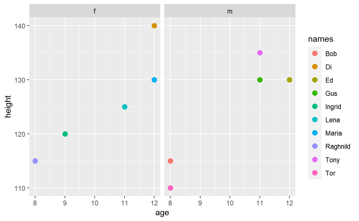
Labels and annotations
Textual labels and annotations (on the plot, axes, geometry, and legend) are an important part of making a plot understandable and communicating information. It is very easy to add such annotations in ggplot:
ggplot(data = kids_frame, aes(x = age, y = height, color = names)) +
  geom_point(size = 3) +
  labs(title = "Height of the kids function of their age",
       subtitle = "The dataset was simulated",
       x = "Age of the kids",
       y = "Height of the kids",
       color = "Names")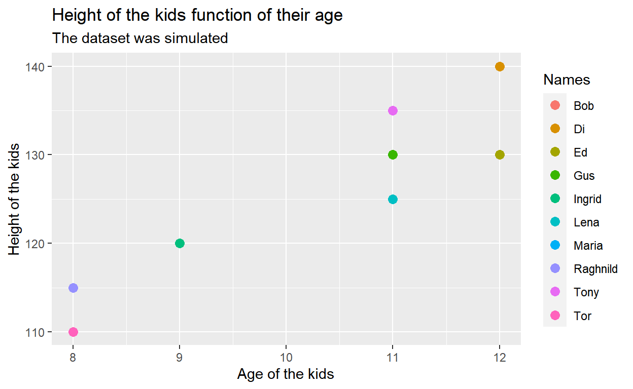
Additional ressources on ggplot2
This lab will get you started with ggplot2. However, this library has much more to offer. If you want to take it further I recommend reading the part I of R for Data Science.
Here is also a cheat sheet so you remember easily the basic functions of ggplot2.
Exercises
Now it is your turn to practice. You will play with the plastic_waste dataset that you can download here:
Note that this is a .csv file, to open it you will need to use the function read.csv():
plastic_waste <- read.csv('C:/Users/benjamcr/Rproj/GEOG3006/data/plastic_waste.csv')The variable descriptions are as follows:
- code: 3 Letter country code
- entity: Country name
- continent: Continent name
- year: Year
- gdp_per_cap: GDP per capita constant 2011 international $, rate
- plastic_waste_per_cap: Amount of plastic waste per capita in kg/day
- mismanaged_plastic_waste_per_cap: Amount of mismanaged plastic waste per capita in kg/day
- mismanaged_plastic_waste: Tonnes of mismanaged plastic waste
- coastal_pop: Number of individuals living on/near coast
- total_pop: Total population according to Gapminder
Question 1: Visualize the relationship between plastic waste per capita and mismanaged plastic waste per capita using a scatterplot. Describe the relationship.
Question 2: Color the points in the scatterplot by continent. Does there seem to be any clear distinctions between continents with respect to how plastic waste per capita and mismanaged plastic waste per capita are associated?
Question 3: Visualize the relationship between plastic waste per capita and total population as well as plastic waste per capita and coastal population. Do either of these pairs of variables appear to be more strongly linearly associated?
Question 4: Recreate the following plot and think about what is wrong about it, how could you make it better?
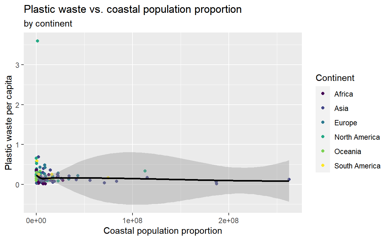
Note that I am using the function scale_color_viridis() from the library viridis.
In next lab we will correct the questions and train more our data vizualisation skills!
Good luck! 💪 💪 💪